Complex Spatial Priors
Michael Stevens
2021-05-26
Source:vignettes/complex-spatial-priors.Rmd
complex-spatial-priors.RmdIntroduction
The geographic profiling models described in the previous tutorials all make use of a Metropolis-Hastings algorithm for updating source locations. As a result, we can impose any prior we like on source locations. So far, priors on source locations have assumed that the probability of observing a source at a specific location is either constant (inside the shapefile) or zero (outside the shapefile). When we update source locations via the Metropolis-Hastings algorithm any proposed value that is outside the shapefile is immediately rejected. This differs from the conventional geographic profiling model (see Verity et al. (2014) and Faulkner et al. (2018)) that implements the shapefile post-hoc. This tutorial will walk through different options for spatial priors in the silverblaze package. Let's start with a refresher: a uniform prior based on simulated data. The prior on source locations is defined over a grid of cells, hence we create a uniform prior via the raster_grid() function.
# define sentinel site array
sentinal_lon <- seq(-0.2, 0.0, l = 15)
sentinal_lat <- seq(51.45, 51.55, l = 15)
sentinal_grid <- expand.grid(sentinal_lon, sentinal_lat)
names(sentinal_grid) <- c("longitude", "latitude")

# create example dataset
data <- sim_data(sentinel_lon = sentinal_grid[,1],
                 sentinel_lat = sentinal_grid[,2],
                 sentinel_radius = 0.3,
                 K = 2,
                 source_lon_min = min(sentinal_lon),
                 source_lon_max = max(sentinal_lon),
                 source_lat_min = min(sentinal_lat),
                 source_lat_max = max(sentinal_lat),
                 sigma_model = "single",
                 sigma_mean = 1,
                 sigma_var = 0,
                 expected_popsize = 1e3)

# store objects for easy access later
df_all <- data$data
dataPoints <- data$record$data_all
true_sources <- data$record$true_source
Now let's create a raster based on the data we've just simulated, this will work as a foundation for our spatial prior.
# create uniform prior on source locations
raster_frame <- raster_grid(cells_lon = 100, cells_lat = 100,
                            range_lat = range(sentinal_lat),
                            range_lon = range(sentinal_lon), guard_rail = 0.25)
This spatial prior is then fed into our geographic profiling project using the spatial_prior argument in the new_set() function. We then specify which kind of prior we wish to impose on source locations, using this raster, via the source_model argument.
# create GP project
p <- rgeoprofile_project()
p <- bind_data(p,
               df = df_all,
               data_type = "counts")

# add parameter set to project
p <- new_set(project = p,
             spatial_prior = raster_frame,
             source_model = "uniform",
             sentinel_radius = 0.3,
             sigma_model = "single",
             sigma_prior_mean = 2,
             sigma_prior_sd = 1,
             expected_popsize_prior_mean = 1e3,
             expected_popsize_prior_sd = 1e2,
             name = "uniform_prior_project")
Now let's have a look at our data and spatial prior.
Bi-variate normal prior
A more informative prior could be a bivariate normal distribution centred on the spatial mean of the positive data. Similarly to Verity et al. (2014), the standard deviation of this bivariate normal prior is set to the maximum distance between the mean and the positive data.
# add parameter set to project
p <- new_set(project = p,
             spatial_prior = raster_frame,
             source_model = "normal",
             sentinel_radius = 0.3,
             sigma_model = "single",
             sigma_prior_mean = 2,
             sigma_prior_sd = 1,
             expected_popsize_prior_mean = 1e3,
             expected_popsize_prior_sd = 1e2,
             name = "bvnorm_prior_project")
Kernel density prior
A bivariate normal distribution may be an inappropriate choice for a prior if the spatial mean of the positive data is an area containing absences. Hence, another option for source_model is "kernel". This will produce a kernel density estimate for the positive data (see Barnard (2010) for a description of the KDE and bandwidth choice).
# add parameter set to project
p <- new_set(project = p,
             spatial_prior = raster_frame,
             source_model = "kernel",
             sentinel_radius = 0.3,
             sigma_model = "single",
             sigma_prior_mean = 2,
             sigma_prior_sd = 1,
             expected_popsize_prior_mean = 1e3,
             expected_popsize_prior_sd = 1e2,
             name = "kde_prior_project")
Using shapefiles
We built our raster from scratch using the raster_grid() function, however, silverblaze also allows for the importing of shapefiles such that the boundaries of our raster conform to a particular geographic boundary. The example here relates to a particular borough of London.
s <- rgeoprofile_shapefile("London_north")## OGR data source with driver: ESRI Shapefile
## Source: "/tmp/RtmpSQHaGH/temp_libpath7377217b642d/silverblaze/extdata/London_north", layer: "boroughs"
## with 8 features
## It has 7 fields
spatial_prior <- raster_from_shapefile(s, cells_lon = 100, cells_lat = 100)
plot(spatial_prior, xlab = "Longitude", ylab = "Latitude")
This shapefile is built into the package, any other shapefile should be loaded using the readOGR() function from rgdal.
A non-uniform spatial prior
There are a lot more shapefiles out there that will provide more information that we might want to influence our model. For example the London Datastore provides shapefiles with various spatial information.
dataStore <- rgeoprofile_shapefile("London_boundary/ESRI")## OGR data source with driver: ESRI Shapefile
## Source: "/tmp/RtmpSQHaGH/temp_libpath7377217b642d/silverblaze/extdata/London_boundary/ESRI", layer: "MSOA_2011_London_gen_MHW"
## with 983 features
## It has 12 fields
print(dataStore)## class : SpatialPolygonsDataFrame
## features : 983
## extent : 503574.2, 561956.7, 155850.8, 200933.6 (xmin, xmax, ymin, ymax)
## crs : +proj=tmerc +lat_0=49 +lon_0=-2 +k=0.999601272 +x_0=400000 +y_0=-100000 +datum=OSGB36 +units=m +no_defs +ellps=airy +towgs84=446.448,-125.157,542.060,0.1502,0.2470,0.8421,-20.4894
## variables : 12
## names : MSOA11CD, MSOA11NM, LAD11CD, LAD11NM, RGN11CD, RGN11NM, USUALRES, HHOLDRES, COMESTRES, POPDEN, HHOLDS, AVHHOLDSZ
## min values : E02000001, Barking and Dagenham 001, E09000001, Barking and Dagenham, E12000007, London, 5184, 5184, 0, 2.9, 2031, 1.6
## max values : E02006931, Westminster 024, E09000033, Westminster, E12000007, London, 14719, 14657, 2172, 247.2, 5936, 3.9Here we see a summary of the data. Lets extract population density from this shapefile and convert it into a raster to use as our spatial prior.
Converting a shapefile to a raster
# Firstly we create a raster that matches the extent of the shapefile.
newRaster <- raster(ncol = 100, nrow = 100)
extent(newRaster) <- extent(dataStore)

# We then rasterize our shapefile using the raster we just created.
PopDenRaster <- rasterize(dataStore, newRaster, field = "POPDEN")

# Finally we project the raster to the correct co-ordinate reference system (CRS).
crs(PopDenRaster) <- crs(dataStore)
PopDenRaster <-  projectRaster(PopDenRaster, crs = "+proj=longlat +datum=WGS84 +ellps=WGS84 +towgs84=0,0,0")
summary(values(PopDenRaster))
## Min. 1st Qu. Median Mean 3rd Qu. Max. NA's
## 2.90 22.50 43.80 51.28 69.20 244.63 7560
# We've obtained our raster, now we need to normalise the population density values so that we're working with probabilities.
values(PopDenRaster) <- values(PopDenRaster)/sum(values(PopDenRaster)[!is.na(values(PopDenRaster))])

# Let's take a look at what the final results.
plot(PopDenRaster, xlab = "Longitude", ylab = "Latitude")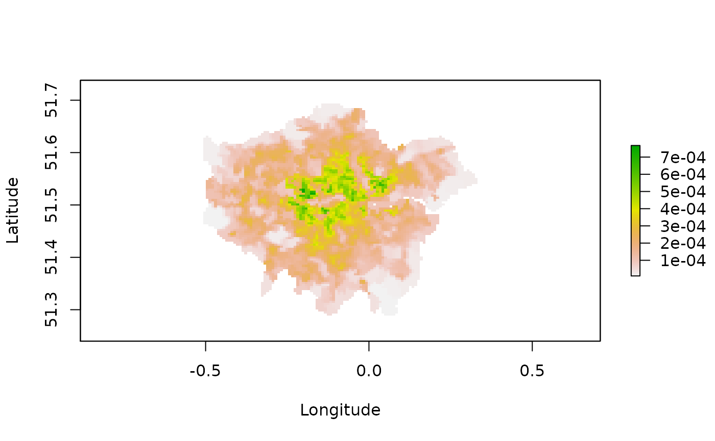
Now we've loaded the shapefile and converted it into a spatial prior, let generate some data, and run the model using the new prior.
A non-uniform spatial prior in a GP project
set.seed(10)
# create example dataset
Extent <- extent(PopDenRaster)
sentGrid <- expand.grid(seq(Extent[1] + 0.1, Extent[2] - 0.1, l = 10), seq(Extent[3]+ 0.05, Extent[4]- 0.05, l = 15))
data <- sim_data(sentinel_lon = sentGrid[,1],
                 sentinel_lat = sentGrid[,2],
                 sentinel_radius = 0.3,
                 K = 2,
                 source_lon_min = Extent[1] + 0.1,
                 source_lon_max = Extent[2] - 0.1,
                 source_lat_min = Extent[3] + 0.05,
                 source_lat_max = Extent[4] - 0.05,
                 sigma_model = "single",
                 sigma_mean = 4,
                 sigma_var = 0,
                 expected_popsize = 1000)
df_all <- data$data
dataPoints <- data$record$data_all
true_sources <- data$record$true_source
Create a geographic profiling project:
pPopDen <- rgeoprofile_project()
pPopDen <- bind_data(pPopDen,
                     df = df_all,
                     data_type = "counts")
Create parameter sets:
# add parameter set to project
pPopDen <- new_set(project = pPopDen,
                   spatial_prior = PopDenRaster,
                   source_model = "manual",
                   sentinel_radius = 0.3,
                   sigma_model = "single",
                   sigma_prior_mean = 4,
                   sigma_prior_sd = 0.1,
                   expected_popsize_prior_sd = 1e3)
## [1] "Using manually specified values in spatial prior"Plot the data with the prior:
Run the MCMC:
set.seed(10)
pPopDen <- run_mcmc(project = pPopDen,
                    K = 1:2,
                    burnin = 2e4,
                    samples = 2e4,
                    pb_markdown = TRUE,
                    converge_test = 1e4)
Plot the prior and the geoprofile:
# uniform
plot3 <- plot_map()
plot3 <- overlay_sources(plot3,
                         lon = true_sources$longitude,
                         lat = true_sources$latitude)

plot3 <- overlay_geoprofile(plot3,
                            pPopDen,
                            K = 2,
                            smoothing = 2,
                            threshold = 1,
                            col = plasma,
                            legend = TRUE)

plot_loglike_diagnostic(pPopDen, K = 2)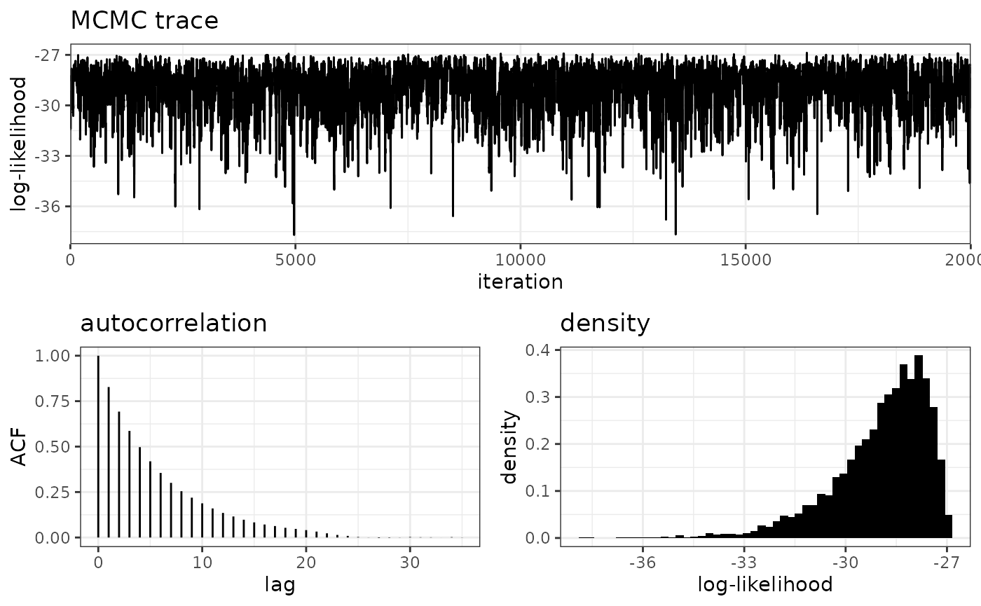
plot3References
Barnard, Etienne. 2010. “Maximum Leave-one-out Likelihood for Kernel Density Estimation.” Proc. of the 21st Annual Symposium of the Pattern Recognition Association, 19–24.
Faulkner, Sally C., Michael C. A. Stevens, Stephanie S. Romañach, Peter A. Lindsey, and Steven C. Le Comber. 2018. “A spatial approach to combatting wildlife crime.” Conservation Biology, 1–24.
Verity, Robert, Mark D. Stevenson, D. Kim Rossmo, Richard A. Nichols, and Steven C. Le Comber. 2014. “Spatial targeting of infectious disease control: Identifying multiple, unknown sources.” Methods in Ecology and Evolution 5 (7): 647–55.