Variable Expected Population

Michael Stevens

2021-05-26

Motivation

An independent expected population model is available within the Silverblaze package but is yet to be investigated. In this tutorial we will generate a couple of toy examples to investigate the following questions:

• Can the model successfully return different population sizes for each source locations?
• How well does the model perform when there is overlap in the dispersal ranges of sources with different sources?

Start by loading the Silverblaze package:

# load packages
library(silverblaze)
# set seed
set.seed(1)

Simple two source example

Setting up and running the independent expected population size model

Set up an array of sentinel sites and a uniform prior. We'll also specify the sentinel site radius.

# sentinel sites
sentinel_lon <- seq(-0.2, 0.0, l = 12)
sentinel_lat <- seq(51.45, 51.55, l = 12)
sentinel_grid <- expand.grid(sentinel_lon, sentinel_lat)
names(sentinel_grid) <- c("longitude", "latitude")

# create source prior
uniform_prior <- raster_grid(cells_lon = 100, cells_lat = 100,
                               range_lat = range(sentinel_lat),
                               range_lon = range(sentinel_lon), guard_rail = 0.5)

# set sentinel radius                               
sentinel_site_radius <- 0.2                               

Now we generate some data. We use the sim_data() function to generate two sources, specifying that each source is responsible for a proportion of the total expected population size setting source_weights = c(0.1, 0.9). This will generate 10% of events around one source, and 90% around another.

sim1 <- sim_data(sentinel_grid$longitude,
                 sentinel_grid$latitude,
                 K = 2,
                 source_weights = c(0.1, 0.9),
                 sigma_model = "single",
                 sigma_mean = 1,      
                 sigma_var = 0,         
                 sentinel_radius = sentinel_site_radius,
                 expected_popsize = 1000)

data_all1 <- sim1$record$data_all
true_source1 <- sim1$record$true_source
K_model <- 2

Now let's build the model parameter set and run the MCMC.

# create a project and bind data
p1 <- rgeoprofile_project()
p1 <- bind_data(p1,
                df = sim1$data,
                data_type = "counts")

# add parameter set to project
p1 <- new_set(project = p1,
              spatial_prior = uniform_prior,
              sentinel_radius = sentinel_site_radius,
              sigma_model = "single",
              sigma_prior_mean = 1,
              sigma_prior_sd = 2,
              expected_popsize_model = "independent", # set model to fit independent EP
              expected_popsize_prior_mean = 500,
              expected_popsize_prior_sd = 250)

plot1 <- plot_map()
plot1 <- overlay_points(plot1, data_all1$lon, data_all1$lat)
plot1 <- overlay_sources(plot1, true_source1$lon, true_source1$lat)
plot1

We can see one source is clearly responsible to generating more data than the other. Let's run the MCMC algorithm. We might expect some mixing issues given the model now needs to estimate independent population sizes. Hence we implement the Metropolis-Hastings coupling protocol.

# optimise beta values for heated MCMC chains with an acceptance prob of at 
# least 0.75.  
beta_k <- optimise_beta(proj = p1, 
                        K = 2, 
                        target_acceptance = 0.75, 
                        max_iterations = 25,
                        beta_init = seq(0,1, l = 10), 
                        coupling_on = TRUE,
                        burnin = 1e3,
                        converge_test = 5e2,
                        samples = 10,
                        create_maps = FALSE,
                        pb_markdown = TRUE)

beta_values <- beta_k$beta_vec[[length(beta_k$beta_vec)]]

# run MCMC under K = 2 model
p1 <- run_mcmc(project = p1,
              K = K_model,
              burnin = 1e4,
              samples = 5e3,
              converge_test = 1e3,
              coupling_on = TRUE, 
              beta_manual = beta_values)

Results

Below we can see the geoprofile of the two sources. By eye it's hard to tell which source has a larger population

# produce and store map
plot1 <- plot_map()
plot1 <- overlay_sentinels(plot1, p1, sentinel_radius = sentinel_site_radius)
plot1 <- overlay_geoprofile(plot1, p1, K = 2)
plot1 <- overlay_sources(plot1, true_source1$lon, true_source1$lat)
plot1

How can we be sure these sigma values are different? We can access the raw output associated to sigma using the get_output() function. We can also look into where our true values fall within the 95% credible intervals of the fitted values.

# get the raw expected population draws
ep_output <- get_output(p1, "expected_popsize_sampling", K = 2, type = "raw")
ep1 <- density(ep_output[,1])
ep2 <- density(ep_output[,2])

# calculate the mean of these draws
estimatedEP <- apply(ep_output, 2, mean)
estimatedEP

##   group1   group2 
## 883.9557 176.9054

plot_expected_popsize(p1, K = 2)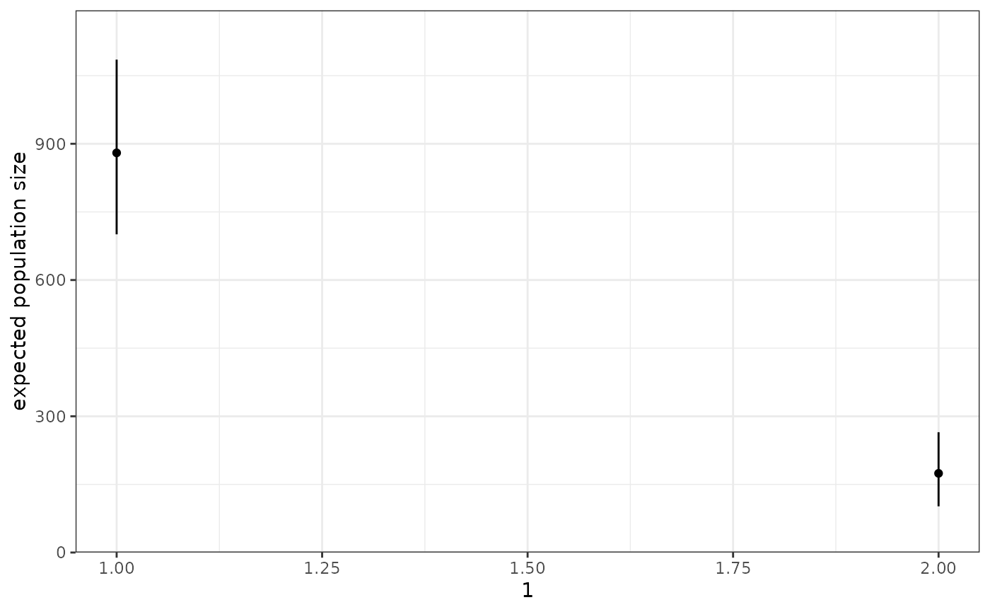

# get the credible intervals for expected popsize
ep_intervals <- get_output(p1, "expected_popsize_intervals", K = 2)
ep_intervals

##            Q2.5     Q50     Q97.5
## group1 700.6451 880.009 1085.2979
## group2 101.7307 174.326  264.8897

As we can see the model is returning the correct proportions of the total expected population size (1000) for each source.

References